Research Projects | 2026
Between the Frameworks
A research case study on teaching AI to see what isn't there: the shadow.
This research stems from a creative challenge: projecting dynamic, ephemeral “virtual skins” onto outdoor physical sculptures over long periods. Existing spatial tracking and computer vision tools rely heavily on controlled studio conditions; sudden shifts in lighting, weather, or faint snowfall routinely break alignment. Furthermore, deploying installations on standalone edge devices meant that heavy vision models hogged the compute needed for real-time rendering.
To solve this, I began developing custom, lightweight Convolutional Neural Networks (CNNs) engineered specifically for edge hardware. The goal is to build an environmental-invariant tracking system—resilient to fluctuating viewpoints, time of day, and weather variations—while leaving the bulk of device processing power free to drive the visual experience.
To solve dynamic tracking, I turned to an equally complex benchmark: tracking shadows. Because shadows continuously stretch, fade, and distort with shifting light, solving this forces a lightweight model to handle dramatic real-world variance.
Why Traditional Computer Vision Fails
Most classical Computer Vision (CV) tools rely on a simple assumption: the object you want to find looks distinctly different from its background. A cat has a different color and texture than a couch, no matter where you photograph it.
Shadows break all of these standard rules:
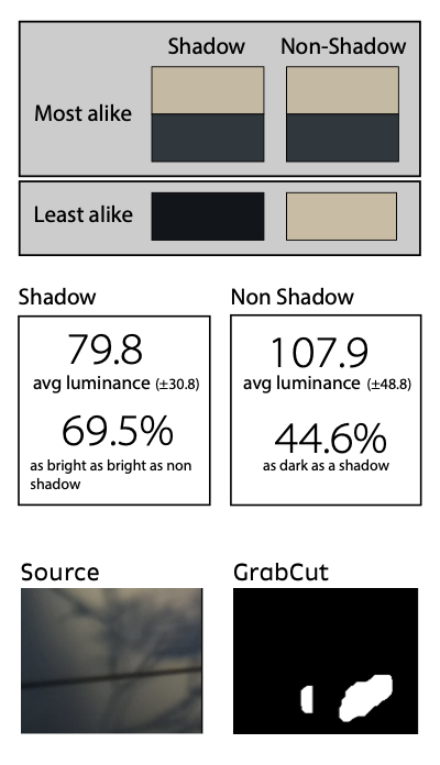
Brightness Thresholds Fail
A shadow on a brightly lit white wall can actually be brighter than an unshaded patch of dark brick right next to it. Simple light-versus-dark cutoffs fall apart immediately.
Color Thresholds Fail
Shadows depending on which surface they are displayed on will vary. Over time their color will change and they dont seperate uniformally from the surface which they apear on
Edge Detection Fails
The Real Task: Isolating the Tree’s Cast Shadow
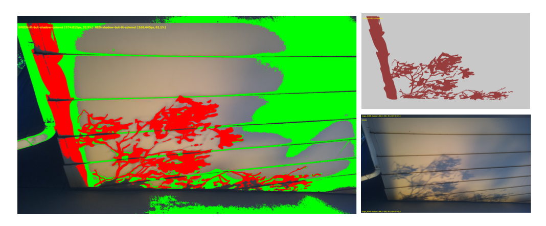
Most tools assume “shadow” is a single global category. In practice, a physical scene contains three distinct, overlapping lighting signals:
• Target Cast Shadow: The specific, high-frequency boundary cast by the subject (e.g., the tree branch).
• Surface/Wall Shading: The inherent gradient or texture of the physical receiver plane.
• Ambient Occlusion: The broad, low-frequency darkening from distant buildings, overhangs, or sky cover.
Generic segmentation tools blur these together or select the entire dark region of the wall. The task here is surgical: isolating the specific cast shadow while ignoring the ambient wall gradient sitting directly beneath it.
How Modern AI Tools Struggle with the Shadow
Segment Anything Model (SAM):
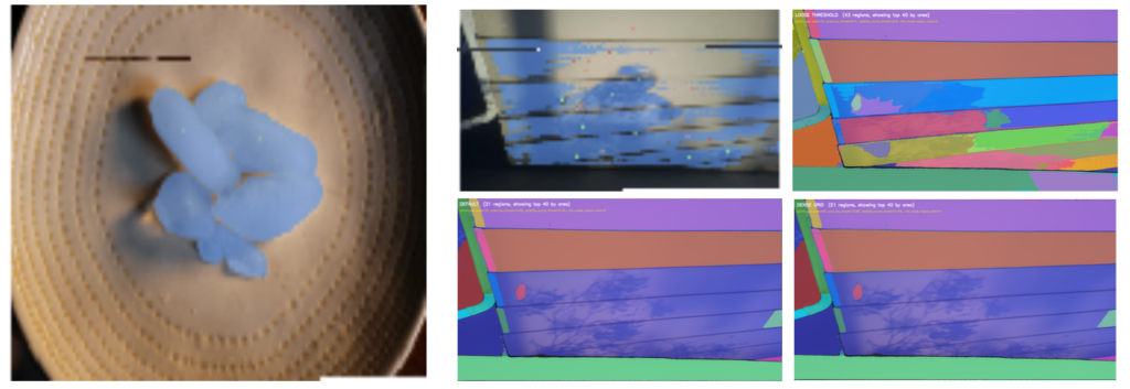
Looking into SAM’s internal attention maps reveals a fundamental structural blind spot: SAM is trained to look for objects, not phenomena.
The Ice Cube Success: SAM excels at segmenting an ice cube because an ice cube is a discrete physical subject with a defined boundary, distinct texture, and clear visual presence.
The Shadow Failure: A shadow is an optical phenomenon painted onto a surface, not an object itself. Because “wall” is a heavily reinforced object class in SAM’s training weights, its attention mechanism
Generative Models (Diffusion & Vision Transformers):
Building The Frame
Understanding why standard AI and computer vision fails at shadows isolation is only half the battle. The real work began in deciding how to fix it.
I don’t have the resources for a single massive, brute-force model which demands enormous amounts of data, computing power, and time. Instead, I approached this as an architectural design problem. My feeling was I could combine the fast precision of traditional algorithms with the more global context of modern deep learning.
What followed was an iterative process of experimentation. I started by pushing custom non-AI pipelines to their limits, mapped out their failure points, and then progressively introduced lightweight, specialized neural networks. Each attempt built upon the lessons of the last, gradually moving toward a modular, distilled system capable of seeing both the tiny pixel details and the bigger picture.
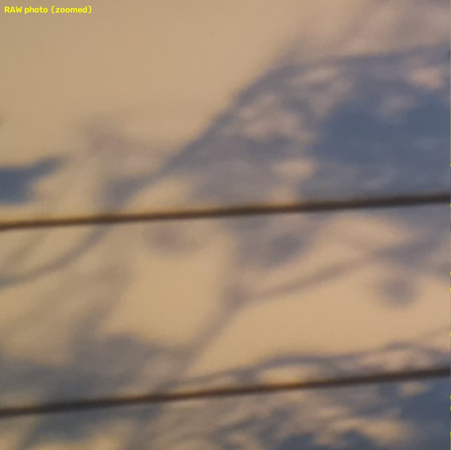
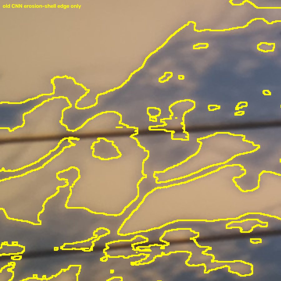
Step 1: Set A baseline using only the foundations.
This system was built without machine learning or neural networks, relying instead on a fundamental rule of optics: a shadow requires both a tonal drop and a corresponding change over time.
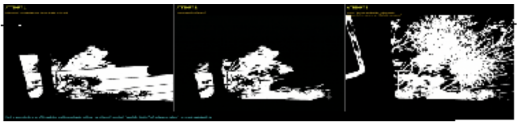
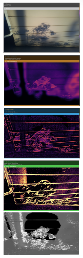
Each of the seven tools analyzed the scene across different spatial scales and windows of time, contributing weighted votes toward a maximum possible score of 38 per pixel:
- Layer 1 Output (Boundary Lock – Tools A & E):
- Layer 2 Output (Penumbra & Fill – Tools B & D):
- Layer 3 Output (Deep Interior – Tool F):
- Layers 4 & 5 Output (Sharpening & Gap Sealing – Tools C & G):
- Final Cascade Consensus (30% Threshold):
What was reassuring is that the entire pipeline was built on pure physics and temporal rules—no manual training, no machine learning weights, and no neural networks.

For an unsupervised, rule-based system built from scratch in two days, this was a massive win. It proved that classical computer vision could capture complex, moving physical structures far better than off-the-shelf tools like GrabCut—setting a strong benchmark for the deep learning models that followed.
Step 2: Transferring Physics to a Lightweight CNN
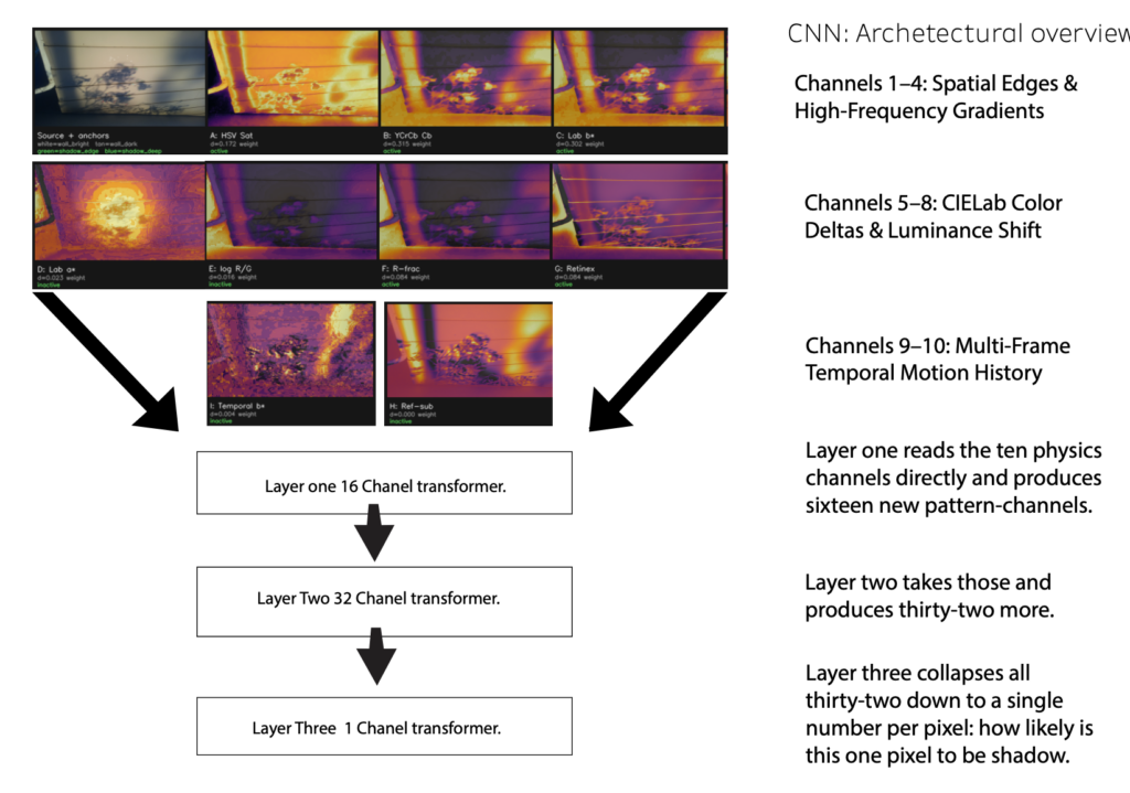
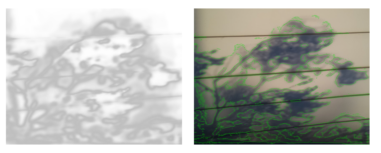
Focusing on small applications of AI with low power use, speed and performance as criteria, I built a hyper-efficient, 3-layer Convolutional Neural Network (CNN) with only 6,129 total parameters. Instead of forcing the network to learn physics from scratch, I fed it a custom 10-channel physics input stack, baking global context, motion, and color logic directly into the inputs before the CNN ever processed a single pixel.
How the Sliding Window Works
Instead of judging each pixel in isolation, the CNN acts as a sliding window across the image:
- Every pixel decision is informed by a 5×5-pixel neighborhood, allowing the network to analyze surrounding spatial patterns.
- Layer 1 reads the 10 physics channels directly to generate 16 pattern maps.
- Layer 2 looks for “patterns within patterns,” expanding to 32 feature channels.
To keep inference fast, the network runs at half-resolution and upscales the final output. During training, I applied 5x edge weighting to the loss function, forcing this tiny 6k-parameter network to focus obsessively on getting the tricky shadow boundaries right.
CNN: Archetectural overview
Channels 1–4: Spatial Edges & High-Frequency Gradients
Channels 5–8: CIELab Color Deltas & Luminance Shift
Channels 9–10: Multi-Frame Temporal Motion History
Layer one reads the ten physics channels directly and produces sixteen new pattern-channels. Layer two takes those and produces thirty-two more. Layer three collapses all thirty-two down to a single number per pixel: how likely is this one pixel to be shadow.
Step 3: Elevating Scene Context with DINOv3 & Self-Supervised Learning
After proving what classical physics rules could do, the next breakthrough meant stepping into modern vision architectures. To give the system true “global awareness”—the ability to understand the whole scene rather than just localized pixels—I integrated DINOv3, a state-of-the-art Vision Transformer (ViT) model. this model is free and can fit on the averaege consumer desktop.
What Makes DINOv3 Different?
Self-Supervised Learning: The model trains itself by looking at millions of unlabeled images, learning the deep structural and geometric relationships of the physical world.
Student-Teacher Distillation: A larger “teacher” network observes an entire image and guides a smaller “student” network to recognize the same underlying structures from cropped or masked views. Over time, the student becomes hyper-efficient at understanding scene context without needing giant datasets.
Attention Routing: the attention maps after fused are then sent though a router where the highest performing values are passed in. The router is a small nureal network design to look at different patterns and build a probability indexed based on the individual layers weights. The router is trained against a few hand drawn truhts
The Breakthrough: Coarse-to-Fine Fusion
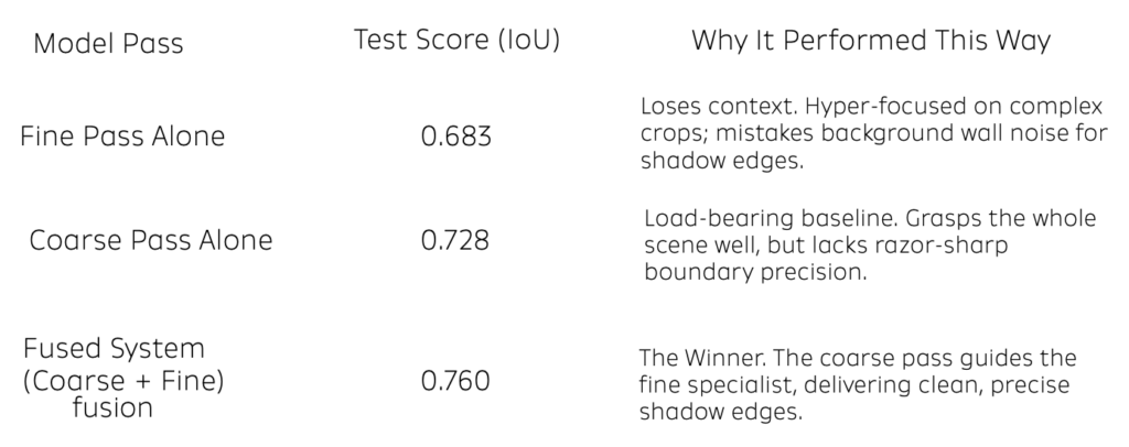
Even with a powerful vision transformer, extracting razor-thin shadow boundaries required a smart sampling strategy. I designed a two-stage Coarse-to-Fine workflow:
The Coarse Pass (The Generalist): Takes a quick, broad look at the entire photo to map out the general shadow boundaries and scene layout.
The Fine Pass (The Specialist): Zooms in only on the fuzzy, high-uncertainty edge crops to evaluate intricate details.
The Fusion Layer: Weighs the coarse prediction against the fine detail prediction, choosing the most reliable score for every pixel.
The Findings: Why the Generalist Must Lead
Testing the sampling passes independently revealed a critical lesson in AI
architecture: specialized models fail when they lose big-picture context.
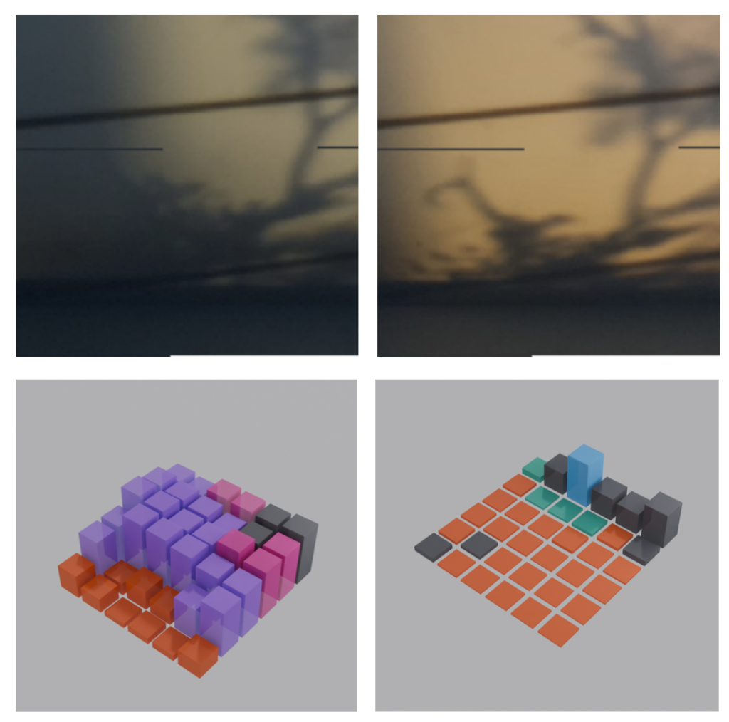
Does the choice of specialist change with the light? Yes.
The channel you’d assume is safe to cut isn’t
Final weight measures output contribution, not necessity
Given sobel’s near-zero final blend weight, the obvious next move is to drop it and simplify the architecture. Tried directly: removing sobel cost real accuracy, despite it barely contributing to the final output.
The explanation is cross-channel self-attention: before any channel’s output gets blended by its tiny final weight, every channel already attended to every other channel and adjusted its own answer using that context. Sobel’s job wasn’t to contribute much of its own signal at the end — it was to calibrate the other channels earlier in the pipeline.
What was Captured
The concrete results, the breakthrough moments, and the unexpected strengths of the model.
Single-Shot Transfer & Focal Depth Intelligence
Without any additional training, the model was tested on a completely new scene—a different tree cast onto a similar wall at a different distance:
In-Focus Shadow Identified: The model crisp-segmented the foreground tree branch shadow sitting directly against the wall.
Background Layer Excluded: Crucially, it completely ignored a secondary, blurry shadow cast by a distant tree further down the wall.
Traditional computer vision tools would have grouped both dark regions together solely based on brightness. The CNN demonstrated a level of focal depth awareness, isolating the primary subject while suppressing layered background noise in a single shot.
Capturing Time: Single-Frame vs. Sequence
Isolating a shadow in a single frame is challenging enough, but watching a model absorb and adapt to a shadow’s behavior over its full temporal duration was unlike anything I had experienced in computer vision.
By processing the sequence over time, the network learned that a shadow is not a static object, but a continuous physical event. As the sun shifted and the shadow deepened, the model dynamically transitioned its confidence from sharp outer edges to deep temporal motion cues.
The Model Out-Annotated the Human
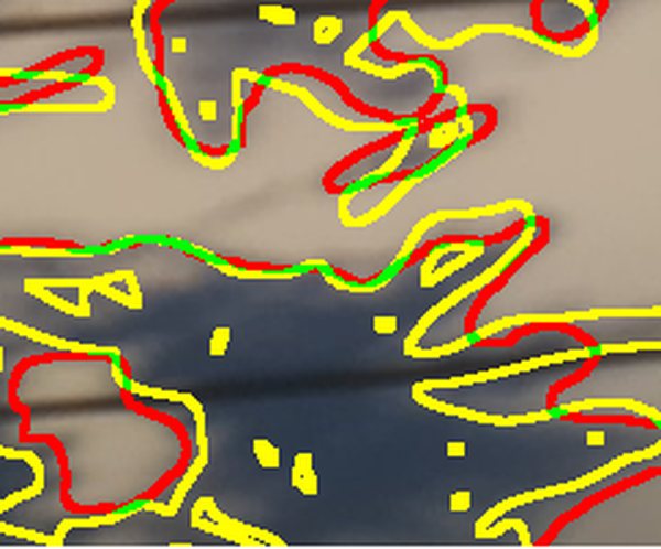
Red is router results
Yellow is hand drawn results
When benchmarking the predictions, a surprising pattern emerged: in several instances, the model’s predicted boundary was more accurate than the hand-drawn “ground truth” mask.
Human annotation of soft, shifting shadows is naturally prone to hand fatigue and subjective error. The model, however, consistently identified sub-pixel tonal transitions that the human eye missed during manual masking. This points toward a powerful future workflow: using early-stage specialized models to bootstrap an
The Student Outperforms the Teacher
2 Million Parameter
0.760: Teacher model, DINOv3 best outcome
6000 Parameter
0.783: Student Model, CNN
By the end of the investigation, the small, custom 6k-parameter CNN actually outscored the massive DINOv3 vision transformer. But it didn’t do so in isolation. The micro-CNN succeeded precisely because DINO’s internal attention weights were extracted and used as a precision reward signal during training.
DINO acted as the global guide; the CNN acted as the hyper-efficient specialist. One model informed the next. This proves that we don’t need gigawatts of compute running at every endpoint—we need small, lightweight models running dynamically at the point of need, handed exact context by an integration layer.
Next Steps & Expanding the Curriculum
A 100-frame sequence of a single tree on one wall was enough to achieve a 0.7835 IoU, but it represents just a fraction of the physical world. Future iterations will focus on expanding the training curriculum:
- Testing curiculium diversification and model capabilities across different times of day
- Evaluating shadows cast across diverse colored and textured walls (brick, wood, painted plaster).
- better quality bootstraps and their effect on training results
- testing the limitations of model diversification within light frame work implementation